Google Sheets Tutorial
The Ultimate Guide to VLOOKUP in Google Sheets
Learn how to master VLOOKUP in Google Sheets with our comprehensive guide. Discover syntax, tips, and use cases.
Table of Contents
VLOOKUP, a cornerstone formula in Google Sheets, empowers you to retrieve data from one table and insert it into another based on a shared value. This seemingly simple formula unlocks a world of possibilities for data analysis and manipulation within your spreadsheets. This comprehensive guide delves into the intricacies of VLOOKUP, transforming you from a VLOOKUP novice to a confident spreadsheet.
Here is a video demonstrating how you can apply VLOOKUP to a Google Sheet:
Why Use VLOOKUP in Google Sheets?
VLOOKUP, though not the only option, stands as a champion formula in Google Sheets for data retrieval. Its widespread use stems from a multitude of advantages that make it a valuable tool for anyone working with spreadsheets. Here's a breakdown of why VLOOKUP deserves a prominent place in your spreadsheet skills:
Simplicity and Ease of Use: VLOOKUP boasts a relatively straightforward syntax compared to some other spreadsheet functions. With a basic understanding of its components (search_key, range, index, [is_sorted]), you can start performing lookups quickly.
Versatility: Enriches data sets, creates dynamic reports, and cleans data.
Efficiency & Automation: VLOOKUP streamlines data analysis workflows. Automating data retrieval through formulas translates to significant time savings compared to manual copy-pasting.
Collaborative Spirit: VLOOKUP thrives in collaboration! It seamlessly integrates with other functions like INDEX, MATCH, and IFERROR. This unlocks even more powerful features like multi-criteria lookups and error handling.
Widespread Use & Support: VLOOKUP's established presence ensures readily available online resources and tutorials. This simplifies troubleshooting and empowers you to explore advanced techniques.
Conditional Lookups: VLOOKUP isn't limited to straightforward data retrieval. When combined with the IFS function, you can create conditional lookups. This empowers you to retrieve different values based on specific criteria within the lookup table, adding another layer of control and decision-making to your spreadsheets.
Formula Auditing and Debugging: VLOOKUP formulas can become complex, especially when combined with other functions. Google Sheets offers a valuable tool called "Formula Auditing." This feature allows you to step through each step of the VLOOKUP formula's evaluation process, pinpointing errors and streamlining the debugging process.
VLOOKUP Syntax
VLOOKUP follows this syntax:
=VLOOKUP(search_key, range, index, [is_sorted])Let's break down each element:
search_key: This is the value you're looking for in the first column of the table you're searching (lookup table). It could be an employee ID, a product code, or any other unique identifier.
range: This is the entire table (including the header row) where you want to find the search_key. Imagine a table containing employee IDs, names, and departments. This entire table would be your range.
index: This specifies the column number within the range table that contains the data you want to retrieve. Perhaps you want to find the corresponding department for a specific employee ID. The index would then point to the column containing department information within the range table.
[is_sorted] (optional): Set to TRUE if the data in your lookup table is sorted in ascending order according to the search_key column. Leaving it blank or setting it to FALSE forces VLOOKUP to perform an exact match regardless of order.
A Step-by-Step Guide to use VLOOKUP in Google Sheets
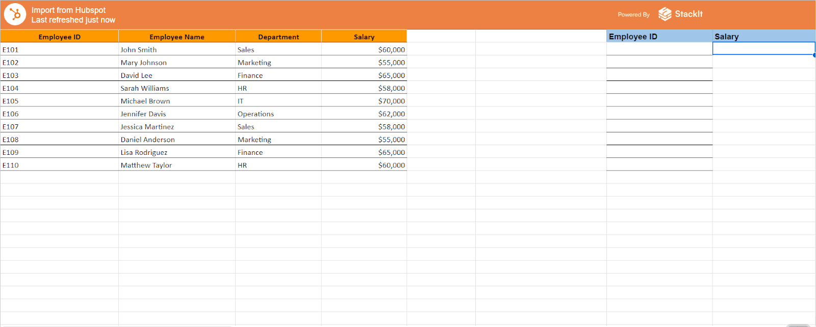
Let's utilize a sample dataset to demonstrate the application of the VLOOKUP function. The dataset provided below has been extracted from HubSpot into Google Sheets using StackIt. For detailed instructions on connecting HubSpot to Google Sheets, please refer to our blog “How to Integrate HubSpot to Google Sheets Seamlessly”.
Imagine you have a table with employee IDs, names, and departments (lookup table), and another table with just employee IDs and corresponding sales figures (data table). You want to find the salary figures for each employee based on their ID. Here's how VLOOKUP can help:
Locate the Formula Bar: Click on the cell where you want the retrieved data to appear in your data table. This is typically an empty cell next to the employee ID in your data table.
Enter the VLOOKUP Formula: =VLOOKUP(
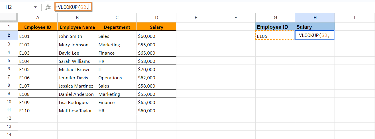
Search Key: Enter the cell reference containing the employee ID from your data table (e.g., G2).
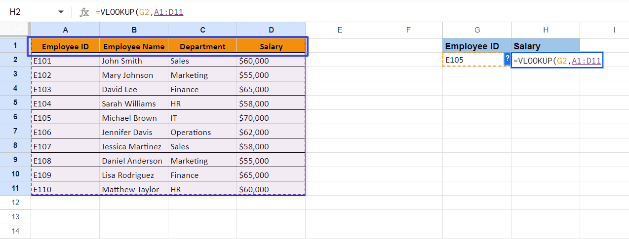
Lookup Table Range: Specify the range of your lookup table, including the header row (e.g., A1:D11). This ensures that VLOOKUP searches the entire table for the employee ID.
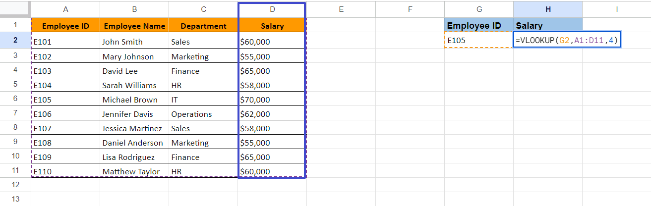
Index: Enter the column number within the lookup table containing the salary figures you want to retrieve (e.g., 4). In this case, the fourth column in your lookup table likely holds the salary figures.
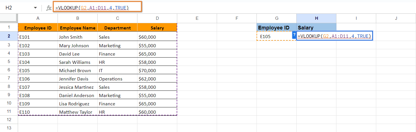
Is Sorted (Optional): If your lookup table (employee ID, name, department) is sorted by employee ID (ascending order), enter TRUE. Otherwise, leave it blank or enter FALSE. VLOOKUP will perform an exact match regardless.
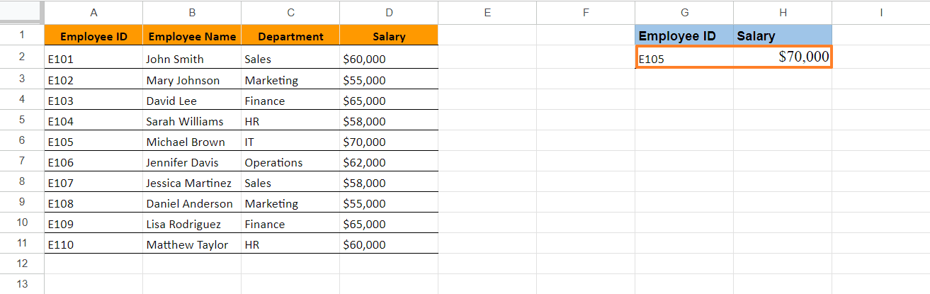
Close the Formula: Press Enter and voila! The corresponding sales figure for the employee ID in cell G2 will appear. This demonstrates the power of VLOOKUP in retrieving data from one table and integrating it into another.
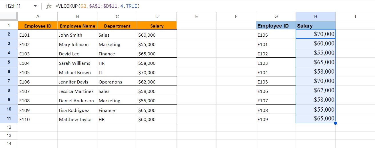
Drag the Formula Down: Drag the formula down to the remaining cells in your data table to automatically populate sales figures for all employees. This is a time-saving technique to populate data across multiple rows.
Bonus Tip: Using Absolute and Relative Cell References
When dragging the formula down, using absolute cell references for the lookup table range (e.g., $A$1:$D$11) ensures the formula always refers to the same lookup table regardless of where it's copied. This prevents errors and simplifies the process.
Considerations to Keep in Mind When Using VLOOKUP in Google Sheets:
Error Handling: VLOOKUP returns the error "#N/A" if the search_key is not found. You can use the IFERROR function to display a custom message or a default value in such cases. This enhances the clarity and robustness of your spreadsheet.
=IFERROR(VLOOKUP(search_key, range, index, FALSE), "Not found")For example, In this formula, if the VLOOKUP function fails to find the search_key in the specified range, it will display "Not found" instead of the "#N/A" error. This ensures a more user-friendly experience for anyone accessing your spreadsheet.
Approximate Matches: By setting is_sorted to FALSE, VLOOKUP performs an exact match. However, you can use wildcards like "*" to find partial matches within the search_key. This can be useful if the exact spelling of the search_key might vary slightly.
Advanced VLOOKUP Techniques
VLOOKUP's versatility extends beyond basic data retrieval. Here are some advanced applications to consider for more complex scenarios:
Multi-criteria Lookups: VLOOKUP excels at finding data based on a single value. But what if you need to search based on multiple criteria? Here's where the magic of combining VLOOKUP with other functions like INDEX and MATCH comes into play. This powerful combination allows you to search for data based on the intersection of multiple conditions, offering greater flexibility for complex lookups.
Dropping the First Row: If your lookup table has a header row containing column labels (e.g., Employee ID, Name, Department), you might not want to include it in the data retrieval process. The ROW() function within VLOOKUP can be your ally in this situation. By incorporating ROW() within the index value, you can effectively adjust the index to exclude the header row during data retrieval.
Potential of Using VLOOKUP in Google Sheets
Utilizing VLOOKUP in Google Sheets, you can streamline data analysis tasks in Google Sheets. Here are some real-world applications:
Enriching Data Sets: Imagine you have a customer list with just email addresses. However, you possess another table containing email addresses and corresponding customer names. VLOOKUP can seamlessly merge these datasets, enriching your customer list with valuable name information.
Creating Dynamic Reports: Reports are often living documents that need to reflect the latest data. VLOOKUP formulas can be embedded within reports to automatically update with changes in your data tables. This ensures your reports always present the most recent information, saving you time and effort.
Data Validation and Cleaning: Inconsistency in data can lead to errors and hinder analysis. VLOOKUP can be a powerful tool for data validation. By comparing values across different tables using VLOOKUP, you can identify discrepancies and inconsistencies, allowing you to clean your data and ensure its accuracy.
Limitations of VLOOKUP
While using VLOOKUP in Google Sheets offers significant capabilities, it's important to be aware of its limitations and considerations to prevent potential errors.
VLOOKUP is not case sensitive: It treats uppercase and lowercase letters as identical. This means that if your lookup value varies in the case from the data in the table, it may not return the expected result.
VLOOKUP does not search columns to the left: Unlike some other lookup functions, VLOOKUP only searches to the right of the specified range. To search columns to the left, you'll need to use an Index Match formula instead.
Sorting requirement with is_sorted set to TRUE: When using VLOOKUP with the is_sorted argument set to TRUE, you must ensure that the first column of the specified range is sorted in ascending order. Failure to do so may lead to incorrect results.
Partial matches using wildcard characters: VLOOKUP can search for partial matches using wildcard characters such as the asterisk (*) and question mark (?). This can be useful for finding approximate matches within your data.
Setting is_sorted to FALSE for exact matches: If you need to return exact matches, especially when using VLOOKUP from another sheet, be sure to set the is_sorted argument to FALSE. This ensures that VLOOKUP searches for an exact match and doesn't rely on sorting.
Single-Criteria Focus (Base Functionality): VLOOKUP inherently searches based on a single value. However, this can be overcome by combining it with other functions for multi-criteria lookups.
Potential Slowdown with Large Datasets: Extremely large lookup tables can hinder spreadsheet performance. Consider alternative functions like INDEX MATCH in such scenarios.
VLOOKUP offers a compelling combination of simplicity, versatility, and efficiency for data retrieval and manipulation in Google Sheets. While it might not be the ultimate solution for every situation, its strengths make it a valuable tool for anyone who wants to streamline data analysis and unlock the potential of their spreadsheets.
Conclusion
This comprehensive guide has equipped you with the knowledge to not only understand VLOOKUP's mechanics but also leverage its power for efficient data retrieval and manipulation. Remember, practice makes perfect. Experiment with VLOOKUP on different datasets, explore its functionalities beyond basic lookups, and don't hesitate to consult the wealth of online resources available. As you refine your VLOOKUP skills, you'll unlock a world of data analysis and automation possibilities within your spreadsheets.
So, the next time you face a data challenge in Google Sheets, remember the power of VLOOKUP. With this newfound knowledge, you can conquer any data hurdle and transform your spreadsheets into insightful tools that drive informed decision-making.
Say goodbye to tedious data exports! 🚀
Are you tired of spending hours manually exporting CSVs from different tools and importing them into Google Sheets?
StackIt is a data connector for Google Sheets that connects your favorite SaaS tools to Google Sheets automatically. You can get data from these platforms into Google Sheets automatically to build reports that update automatically.
Bid farewell to tedious exports and repetitive tasks. With StackIt, you can add 1 additional day to your week. Try StackIt out for free or schedule a demo.
VLOOKUP, a cornerstone formula in Google Sheets, empowers you to retrieve data from one table and insert it into another based on a shared value. This seemingly simple formula unlocks a world of possibilities for data analysis and manipulation within your spreadsheets. This comprehensive guide delves into the intricacies of VLOOKUP, transforming you from a VLOOKUP novice to a confident spreadsheet.
Here is a video demonstrating how you can apply VLOOKUP to a Google Sheet:
Why Use VLOOKUP in Google Sheets?
VLOOKUP, though not the only option, stands as a champion formula in Google Sheets for data retrieval. Its widespread use stems from a multitude of advantages that make it a valuable tool for anyone working with spreadsheets. Here's a breakdown of why VLOOKUP deserves a prominent place in your spreadsheet skills:
Simplicity and Ease of Use: VLOOKUP boasts a relatively straightforward syntax compared to some other spreadsheet functions. With a basic understanding of its components (search_key, range, index, [is_sorted]), you can start performing lookups quickly.
Versatility: Enriches data sets, creates dynamic reports, and cleans data.
Efficiency & Automation: VLOOKUP streamlines data analysis workflows. Automating data retrieval through formulas translates to significant time savings compared to manual copy-pasting.
Collaborative Spirit: VLOOKUP thrives in collaboration! It seamlessly integrates with other functions like INDEX, MATCH, and IFERROR. This unlocks even more powerful features like multi-criteria lookups and error handling.
Widespread Use & Support: VLOOKUP's established presence ensures readily available online resources and tutorials. This simplifies troubleshooting and empowers you to explore advanced techniques.
Conditional Lookups: VLOOKUP isn't limited to straightforward data retrieval. When combined with the IFS function, you can create conditional lookups. This empowers you to retrieve different values based on specific criteria within the lookup table, adding another layer of control and decision-making to your spreadsheets.
Formula Auditing and Debugging: VLOOKUP formulas can become complex, especially when combined with other functions. Google Sheets offers a valuable tool called "Formula Auditing." This feature allows you to step through each step of the VLOOKUP formula's evaluation process, pinpointing errors and streamlining the debugging process.
VLOOKUP Syntax
VLOOKUP follows this syntax:
=VLOOKUP(search_key, range, index, [is_sorted])Let's break down each element:
search_key: This is the value you're looking for in the first column of the table you're searching (lookup table). It could be an employee ID, a product code, or any other unique identifier.
range: This is the entire table (including the header row) where you want to find the search_key. Imagine a table containing employee IDs, names, and departments. This entire table would be your range.
index: This specifies the column number within the range table that contains the data you want to retrieve. Perhaps you want to find the corresponding department for a specific employee ID. The index would then point to the column containing department information within the range table.
[is_sorted] (optional): Set to TRUE if the data in your lookup table is sorted in ascending order according to the search_key column. Leaving it blank or setting it to FALSE forces VLOOKUP to perform an exact match regardless of order.
A Step-by-Step Guide to use VLOOKUP in Google Sheets
Let's utilize a sample dataset to demonstrate the application of the VLOOKUP function. The dataset provided below has been extracted from HubSpot into Google Sheets using StackIt. For detailed instructions on connecting HubSpot to Google Sheets, please refer to our blog “How to Integrate HubSpot to Google Sheets Seamlessly”.
Imagine you have a table with employee IDs, names, and departments (lookup table), and another table with just employee IDs and corresponding sales figures (data table). You want to find the salary figures for each employee based on their ID. Here's how VLOOKUP can help:
Locate the Formula Bar: Click on the cell where you want the retrieved data to appear in your data table. This is typically an empty cell next to the employee ID in your data table.
Enter the VLOOKUP Formula: =VLOOKUP(
Search Key: Enter the cell reference containing the employee ID from your data table (e.g., G2).
Lookup Table Range: Specify the range of your lookup table, including the header row (e.g., A1:D11). This ensures that VLOOKUP searches the entire table for the employee ID.
Index: Enter the column number within the lookup table containing the salary figures you want to retrieve (e.g., 4). In this case, the fourth column in your lookup table likely holds the salary figures.
Is Sorted (Optional): If your lookup table (employee ID, name, department) is sorted by employee ID (ascending order), enter TRUE. Otherwise, leave it blank or enter FALSE. VLOOKUP will perform an exact match regardless.
Close the Formula: Press Enter and voila! The corresponding sales figure for the employee ID in cell G2 will appear. This demonstrates the power of VLOOKUP in retrieving data from one table and integrating it into another.
Drag the Formula Down: Drag the formula down to the remaining cells in your data table to automatically populate sales figures for all employees. This is a time-saving technique to populate data across multiple rows.
Bonus Tip: Using Absolute and Relative Cell References
When dragging the formula down, using absolute cell references for the lookup table range (e.g., $A$1:$D$11) ensures the formula always refers to the same lookup table regardless of where it's copied. This prevents errors and simplifies the process.
Considerations to Keep in Mind When Using VLOOKUP in Google Sheets:
Error Handling: VLOOKUP returns the error "#N/A" if the search_key is not found. You can use the IFERROR function to display a custom message or a default value in such cases. This enhances the clarity and robustness of your spreadsheet.
=IFERROR(VLOOKUP(search_key, range, index, FALSE), "Not found")For example, In this formula, if the VLOOKUP function fails to find the search_key in the specified range, it will display "Not found" instead of the "#N/A" error. This ensures a more user-friendly experience for anyone accessing your spreadsheet.
Approximate Matches: By setting is_sorted to FALSE, VLOOKUP performs an exact match. However, you can use wildcards like "*" to find partial matches within the search_key. This can be useful if the exact spelling of the search_key might vary slightly.
Advanced VLOOKUP Techniques
VLOOKUP's versatility extends beyond basic data retrieval. Here are some advanced applications to consider for more complex scenarios:
Multi-criteria Lookups: VLOOKUP excels at finding data based on a single value. But what if you need to search based on multiple criteria? Here's where the magic of combining VLOOKUP with other functions like INDEX and MATCH comes into play. This powerful combination allows you to search for data based on the intersection of multiple conditions, offering greater flexibility for complex lookups.
Dropping the First Row: If your lookup table has a header row containing column labels (e.g., Employee ID, Name, Department), you might not want to include it in the data retrieval process. The ROW() function within VLOOKUP can be your ally in this situation. By incorporating ROW() within the index value, you can effectively adjust the index to exclude the header row during data retrieval.
Potential of Using VLOOKUP in Google Sheets
Utilizing VLOOKUP in Google Sheets, you can streamline data analysis tasks in Google Sheets. Here are some real-world applications:
Enriching Data Sets: Imagine you have a customer list with just email addresses. However, you possess another table containing email addresses and corresponding customer names. VLOOKUP can seamlessly merge these datasets, enriching your customer list with valuable name information.
Creating Dynamic Reports: Reports are often living documents that need to reflect the latest data. VLOOKUP formulas can be embedded within reports to automatically update with changes in your data tables. This ensures your reports always present the most recent information, saving you time and effort.
Data Validation and Cleaning: Inconsistency in data can lead to errors and hinder analysis. VLOOKUP can be a powerful tool for data validation. By comparing values across different tables using VLOOKUP, you can identify discrepancies and inconsistencies, allowing you to clean your data and ensure its accuracy.
Limitations of VLOOKUP
While using VLOOKUP in Google Sheets offers significant capabilities, it's important to be aware of its limitations and considerations to prevent potential errors.
VLOOKUP is not case sensitive: It treats uppercase and lowercase letters as identical. This means that if your lookup value varies in the case from the data in the table, it may not return the expected result.
VLOOKUP does not search columns to the left: Unlike some other lookup functions, VLOOKUP only searches to the right of the specified range. To search columns to the left, you'll need to use an Index Match formula instead.
Sorting requirement with is_sorted set to TRUE: When using VLOOKUP with the is_sorted argument set to TRUE, you must ensure that the first column of the specified range is sorted in ascending order. Failure to do so may lead to incorrect results.
Partial matches using wildcard characters: VLOOKUP can search for partial matches using wildcard characters such as the asterisk (*) and question mark (?). This can be useful for finding approximate matches within your data.
Setting is_sorted to FALSE for exact matches: If you need to return exact matches, especially when using VLOOKUP from another sheet, be sure to set the is_sorted argument to FALSE. This ensures that VLOOKUP searches for an exact match and doesn't rely on sorting.
Single-Criteria Focus (Base Functionality): VLOOKUP inherently searches based on a single value. However, this can be overcome by combining it with other functions for multi-criteria lookups.
Potential Slowdown with Large Datasets: Extremely large lookup tables can hinder spreadsheet performance. Consider alternative functions like INDEX MATCH in such scenarios.
VLOOKUP offers a compelling combination of simplicity, versatility, and efficiency for data retrieval and manipulation in Google Sheets. While it might not be the ultimate solution for every situation, its strengths make it a valuable tool for anyone who wants to streamline data analysis and unlock the potential of their spreadsheets.
Conclusion
This comprehensive guide has equipped you with the knowledge to not only understand VLOOKUP's mechanics but also leverage its power for efficient data retrieval and manipulation. Remember, practice makes perfect. Experiment with VLOOKUP on different datasets, explore its functionalities beyond basic lookups, and don't hesitate to consult the wealth of online resources available. As you refine your VLOOKUP skills, you'll unlock a world of data analysis and automation possibilities within your spreadsheets.
So, the next time you face a data challenge in Google Sheets, remember the power of VLOOKUP. With this newfound knowledge, you can conquer any data hurdle and transform your spreadsheets into insightful tools that drive informed decision-making.
Say goodbye to tedious data exports! 🚀
Are you tired of spending hours manually exporting CSVs from different tools and importing them into Google Sheets?
StackIt is a data connector for Google Sheets that connects your favorite SaaS tools to Google Sheets automatically. You can get data from these platforms into Google Sheets automatically to build reports that update automatically.
Bid farewell to tedious exports and repetitive tasks. With StackIt, you can add 1 additional day to your week. Try StackIt out for free or schedule a demo.
FAQs
What are some alternatives to VLOOKUP?
What are some alternatives to VLOOKUP?
Can I use VLOOKUP to perform calculations on retrieved data?
Can I use VLOOKUP to perform calculations on retrieved data?
Is there a limit to the size of the lookup table I can use with VLOOKUP?
Is there a limit to the size of the lookup table I can use with VLOOKUP?
Automatic Data Pulls
Visual Data Preview
Set Alerts
other related blogs
Try it now